There are 7 ordinary differential equation initial value problem solvers in MATLAB:
- ode45
- ode23
- ode113
- ode15s
- ode23s
- ode23t
- ode23tb
To choose between the solvers, it's first necessary to understand why one solver might be better than another for a given problem.
The ODE solvers in MATLAB all work on initial value problems of the form,
Starting with the initial conditions
Theoretically, this numerical solution technique is possible because of the connection between differential equations and integrals provided by the fundamental theorem of calculus:
Example: Euler's Method
Euler's method is a simple ODE solver, but it provides an illustration of the trade-offs between efficiency and accuracy in an ODE solver algorithm. Suppose you want to solveNot really. The exact solution to this equation is

Improving on Euler's Method
Using smaller and smaller step sizes turns out to not be a good idea, since the algorithm loses efficiency. For any reasonable problem such a solver would be very slow. Also, Euler's method has a few inherent problems. Since the slope ofSophisticated ODE solvers, like the ones in MATLAB, also estimate the error in each step to determine how big the next step size should be. This is another improvement over the fixed step sizes used above, since a solver that does more work per step is able to compensate by taking steps of varying size. The error estimate used to determine the step size is typically obtained by comparing the results of two different methods. MATLAB's ODE solvers follow a naming convention that reveals information about which methods they use. ode45 compares the results of a 4th-order Runge-Kutta method and a 5th-order Runge-Kutta method to determine the error. Similarly, ode23 uses a 2nd-order and 3rd-order Runge-Kutta comparison. So, in general, the smaller the number odeNN, the looser the solver's error tolerance is.
It should be no surprise, then, that ode45 obtains a very accurate answer for the equation we solved before with Euler's method. ode45 is MATLAB's general purpose ODE solver, and it is the first solver you should use for most problems.
y = @(t) t.^2; x = linspace(0,3); figure plot(x,y(x)) xlabel('t'), ylabel('y(t)') hold on [t,y] = ode45(@(t,y) 2*t, [0 3], 0); plot(t,y,'o') xlabel('t'), ylabel('y(t)') title('Solution of y''=2t using ode45')

Stiff Differential Equations
For some ODE problems, the step size taken by the solver is forced down to an unreasonably small level in comparison to the interval of integration, even in a region where the solution curve is smooth. These step sizes can be so small that traversing a short time interval might require millions of evaluations. This can lead to the solver failing the integration, but even if it succeeds it will take a very long time to do so.Equations that cause this behavior in ODE solvers are said to be stiff. This is a nod to the fact that the equations are stubborn and not easily evaluated with numerical techniques. The problem that stiff ODEs pose is that explicit solvers (such as ode45) are untenably slow in achieving a solution. This is why ode45 is classified as a nonstiff solver along with ode23 and ode113. These solvers all struggle to integrate stiff equations.
Equation stiffness resists a precise definition, because there are several factors that cause it. Stiffness results from a combination of the specific equations, the ODE solver being used, the initial conditions, and the error tolerance used by the solver. The following statements about stiffness, attributed to Lambert [6], are exhibited by many examples of stiff ODEs, but counterexamples also exist, so they are not true definitions of stiffness:
- A linear constant coefficient system is stiff if all of its eigenvalues have negative real part and the stiffness ratio [of the largest and smallest eigenvalues] is large.
- Stiffness occurs when the mathematical problem is stable, and yet stability requirements, rather than those of accuracy, severely constrain the step length.
- Stiffness occurs when some components of the solution decay much more rapidly than others.
For example, equations describing chemical reactions frequently display stiffness, since it is common for components of the solution to vary on drastically different time scales (reactions occurring at the same time that are both very slow and very fast).
However, there are solvers specifically designed to work on stiff ODEs. Solvers that are designed for stiff problems typically do more work per step, and the pay-off is that they are able to take much larger steps and enjoy improved numerical stability compared to the nonstiff solvers. Stiff solvers are implicit, because the computation of
This is just a cursory treatment of stiffness, because it is a complex topic. See Ordinary Differential Equations: Stiffness for a more in-depth look.
To summarize, the nonstiff solvers in MATLAB are:
- ode45
- ode23
- ode113
- ode15s
- ode23s
- ode23t
- ode23tb
Solver Recommendations
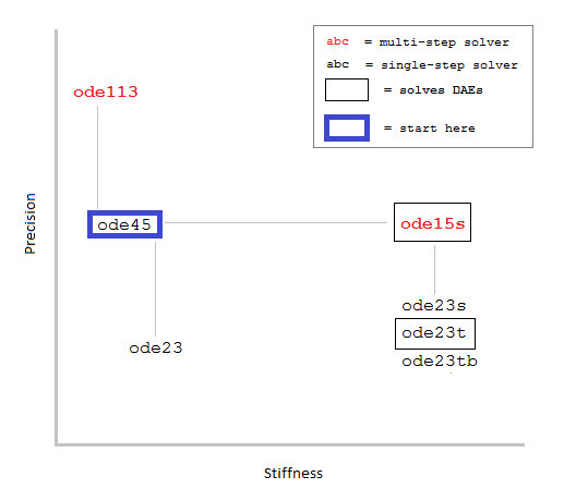
The following recommendations are adapted from the MATLAB Mathematics documentation :- ode45 is MATLAB's general purpose single-step ODE solver. This should be the first solver you use for most problems.
- ode23 is another single-step solver that can be more efficient than ode45 if the problem permits a crude error tolerance. This looser error tolerance can also accommodate some mildly stiff problems.
- ode113 is a multi-step solver, and is preferred over ode45 if the function is expensive to evaluate, or for smooth problems where high precision is required. For example, ode113 excels with orbital dynamics and celestial mechanics problems.
- ode15s is a multi-step solver that is MATLAB's general purpose solver for stiff problems. Use ode15s if ode45 fails or struggles to complete the integration in a reasonable amount of time. ode15s is also the primary solver for DAEs, which are identified as ODEs with a singular mass matrix.
- For stiff problems with crude error tolerances, ode23s, ode23t, and ode23tb provide more efficient alternatives to ode15s since they are single-step solvers. The efficiency of ode23s can be significantly improved by providing the Jacobian, since ode23s evaluates the Jacobian in each step.
- ode23s only works on ODEs with a mass matrix if the mass matrix is constant (not time- or state-dependent).
- ode15s and ode23t are the only solvers that solve DAEs of index 1.
Example 1: Damped Pendulum
The equation of motion for a damped pendulum is,Some natural initial conditions would be
The file pendulumODE.m reformulates the problem as a coupled system of first-order ODEs:
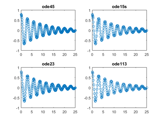
The solvers all perform well, but the damped pendulum is a good example of a nonstiff problem where ode45 performs nicely. In this case ode15s needs to do extra work in order to achieve an inferior solution.
Example 2: van der Pol Oscillator
The van der Pol Oscillator equation becomes stiff in certain intervals when the nonlinear parameterAttempting to solve this equation using ode45 is met with severe resistance, requiring millions of evaluations and 30+ minutes of execution (I stopped execution after 35 minutes). Since the problem is clearly stiff, this example compares the stiff solvers.
The file vanderpolODE.m finds the solution for
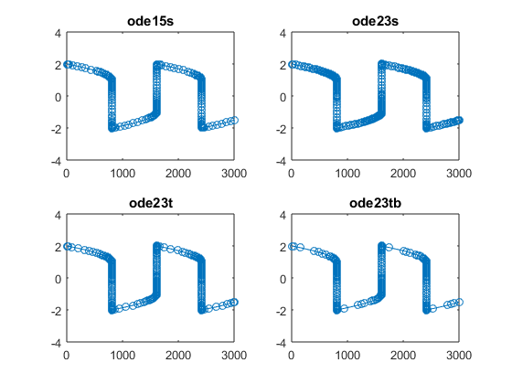
The plots are of the solutions for y1 . For this problem, ode23s executes quickest and with the least number of failed steps. The supplied Jacobian greatly assists ode23s in evaluating the partial derivatives in each step. ode23tb also solves the problem with the fewest number of steps, outperforming ode15s. This problem is a good example of a stiff problem with a crude tolerance where ode23s and ode23tb can out perform ode15s.
But practically speaking, all of the stiff solvers perform well on this
problem and offer significant time savings when compared to ode45.
Sign up here with your email
ConversionConversion EmoticonEmoticon